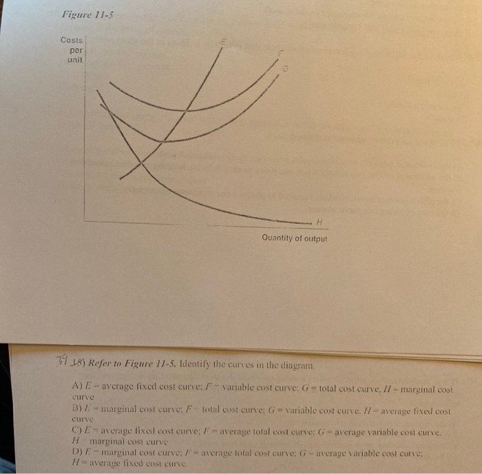
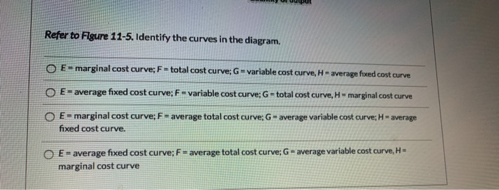
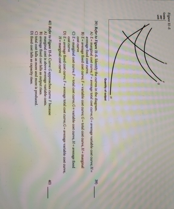
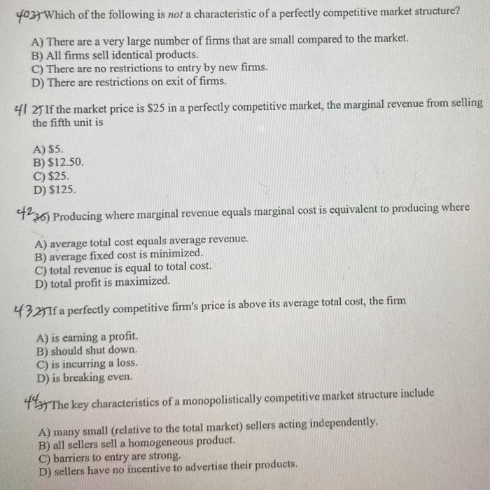
44 refer to figure 11-5. identify the curves in the diagram.
Figure 13-16. 58) Refer to Figure 13-16. Figure 13-16 depicts a monopolistically competitive barber shop. Use the diagram to answer the following questions. a. Suppose the average variable cost of production is $15 when output equals 110 haircuts and $15.25 when output equals 140 haircuts. 10) Refer to Figure 12-5. Economies of scale are exhausted at which output level? A) Q 1 units. B) Q 2 units. C) Q 3 units. D) more than Q 1 units. 11) Refer to Figure 12-5. If the diagram represents a typical firm in the market, what is likely to happen in the long run? A) Competition will be intensified as firms strive to make long run profits.
9) Refer to Figure 9-5. Which of the following statements is true? A) Bundles r and w are not affordable. B) The consumer gets less utility from bundle w than from bundle v. C) Bundles r, s, t and u all cost the same. D) The consumer gets more utility from bundle r than from bundle v. 10) Refer to Figure 9-5.
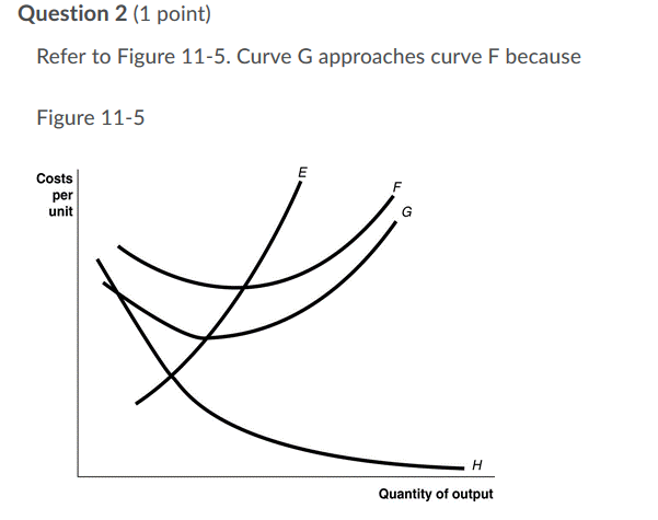
Refer to figure 11-5. identify the curves in the diagram.
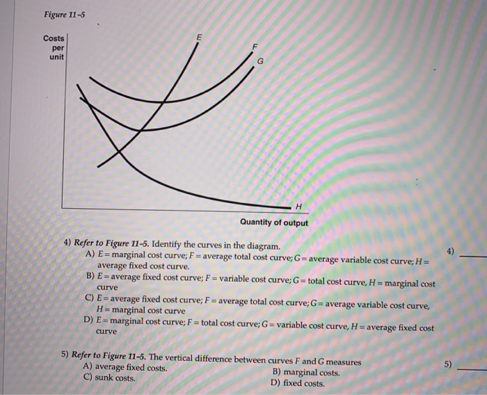
Figure 11-7 Figure 11-7 shows the cost structure for a firm. 23) Refer to Figure 11-7. When the output level is 100 units average fixed cost is 23) A) $10. B) $8. C) $5. D) This cannot be determined from the diagram. Refer to Figure 3 above Identify the curves in the diagram: A) E = average fixed cost curve; F = variable cost curve; G = total cost curve, marginal cost curve. B) E = marginal cost curve; F = total cost curve; G = variable cost curve, H = average fixed cost curve. Refer to Figure 11-5. Identify the curves in the diagram. -E = marginal cost curve; F = total cost curve; G = variable cost curve, H = average fixed cost curve
Refer to figure 11-5. identify the curves in the diagram.. Refer to Figure 11-5. Identify the curves in the diagram. ... Refer to Figure 11-5. The vertical difference between curves F and G measures. average fixed costs. 1. If average total cost is $50 and average fixed cost is $15 when output is 20 units, then the firm's total variable cost at that level of output is. Refer to Figure 11-5. Identify the curves in the diagram. A) E = average fixed cost curve; F = average total cost curve; G = average variable cost curve, H = marginal cost curve. B) E = marginal cost curve; F = total cost curve; G = variable cost curve, H = average fixed cost curve. C) E = average fixed cost curve; F = variable cost curve; G ... Transcribed image text: Refer to Figure 11-5, Identify the curves in the diagram. A) E = marginal cost curves F = average total cost curve; G = average variable cost curve; H = average fixed cost curve. pts Figure 2 14 Refer to Figure 2 14 Identify the two arrows in the diagram from ECO 2023 at Florida International University. ... Identify the two arrows in the diagram that depict the following transaction: ... they both refer to a shift of the demand curve.
In the above diagram curves 12 and 3 represent the. A firms total product curve shows. Refer to the above data. The total output of a firm will be at a maximum where. ... Econhwsols7 Pdf 22 Award 1 00 Point Refer To The Diagram Total ... Refer To Figure 11 5 Identify The Curves In The Di... average fixed cost curve. 21) Refer to Figure 11 -5. The vertical difference between curves F and G measures 21) A) marginal costs. B) fixed costs. C) average fixed costs. D) sunk costs. 22) Refer to Figure 11 -5. Curve G approaches curve F because 22) A) fixed cost falls as capacity rises. B) total cost falls as more and more is produced. May 17, 2015 — Identify the curves in the diagram. G average variable cost curve. E marginal cost curve. 17 refer to figure 11 5. 7 refer to figure 11 5. Figure 2 shows the cost curves for a typical firm. For a given price (such as P*), the level of output that maximizes profit is the output where marginal ...
Figure 11 -4 7) Refer to Figure 11 -4. What happens to the average fixed cost of production when the firm increases ... In a diagram showing the average total cost and average variable cost curves, the minimum point ... Figure 12 -5 Figure 12 - 5 shows cost and demand curves facing a typical firm in a constant - cost, perfectly competitive ... C) explains why the average total cost and marginal cost curves are U-shaped in ... Figure 11-517) Refer to Figure 11-5. ... 22) Refer to the above graph. Refer to Figure 11-5. Curve G approaches curve F because a)total cost falls as more and more is produced. b)marginal cost is above average variable costs c)fixed cost falls as capacity rises. d)average fixed cost falls as output rises. d. Refer to Figure 11-5. Identify the curves in the diagram. a)E = marginal cost curve; F = total cost curve ... Whether the intersection is located on a curve (see FDM 11-25-2.9) ... Figure 1.3 Conflict point Diagrams for expressway T-intersections10.
Solved Question 2 1 Point Refer To Figure 11 5 Curve G Chegg Com
Figure 11-7 Figure 11-7 shows the cost structure for a firm. Refer to Figure 11-7. When the output level is 100 units average fixed cost is A. $10. B. $8. C. $5. D. This cannot be determined from the diagram.

Seasonal Variation Of The Indonesian Throughflow In Makassar Strait In Journal Of Physical Oceanography Volume 42 Issue 7 2012
In Figure 8.1, diagram "a" presents the cost curves that are relevant to a firm's production decision, and diagram "b" shows the market demand and supply curves for the market. Use both diagrams to answer the indicated questions. Figure 8.1
Refer To Figure 11 5 Identify The Curves In The Diagram Wiring Site Resource
Refer to figure 11 5 identify the curves in the. 18) Refer to Figure 11 - 5. Identify the curves in the diagram. A) E = marginal cost curve; F = average total cost curve; G = average variable cost curve; average fixed cost curve. B) E = average fixed cost curve; F = variable cost curve; G = total cost curve, H = marginal cost curve C) E ...
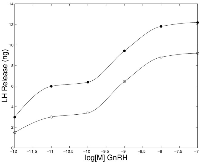
A Mathematical Model For Lh Release In Response To Continuous And Pulsatile Exposure Of Gonadotrophs To Gnrh Theoretical Biology And Medical Modelling Full Text
Consider the phase diagram for carbon dioxide shown in Figure 5 as another example. The solid-liquid curve exhibits a positive slope, indicating that the melting point for CO 2 increases with pressure as it does for most substances (water being a notable exception as described previously). Notice that the triple point is well above 1 atm, indicating that carbon dioxide cannot exist as a liquid ...
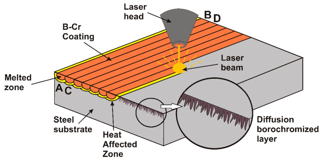
Coatings Free Full Text Microstructural And Mechanical Properties Of B Cr Coatings Formed On 145cr6 Tool Steel By Laser Remelting Of Diffusion Borochromized Layer Using Diode Laser Html
Explain how the law of diminishing returns influences the shapes of the total variable-cost and total-cost curves. b. Graph AFC, AVC, ATC, and MC. Explain the ...
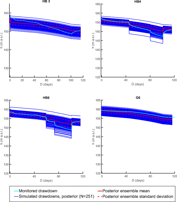
Ensemble Based Stochastic Permeability And Flow Simulation Of A Sparsely Sampled Hard Rock Aquifer Supported By High Performance Computing Springerlink
Refer to Figure 11-5. Identify the curves in the diagram. $8. Figure 11-7 shows the cost structure for a firm. Refer to Figure 11-7. When the output level is 100 units, average fixed cost is. ... Refer to Figure 11-11. For output rates greater than 20,000 picture frames per month,

The Annual Cycle Of Sst In The Eastern Tropical Pacific Diagnosed In An Ocean Gcm In Journal Of Climate Volume 11 Issue 5 1998
Suppose the new situation has price levels Px = $5 and Py = $5 (this is our "situation 3"). In this case, the individual consumes X=1 and Y=3. Using this information, along with the information provided for situation 1, derive the demand curve for Y. (Assume that the demand curve for Y is a straight line.) ANSWER: a and b. The graph is as ...
2
Production Function and TP Curve for George and Martha's Farm. Although the total product curve in the figure slopes upward along its entire.Missing: identify | Must include: identify

Experimental Study On Swelling Behaviour And Microstructure Changes Of Natural Stiff Teguline Clays Upon Wetting
Refer to Figure 11-5. Identify the curves in the diagram. -E = marginal cost curve; F = total cost curve; G = variable cost curve, H = average fixed cost curve
Solved Figure 15 2 Price And Cost Per Unit P Mc Ato Ps Latc Chegg Com
Refer to Figure 3 above Identify the curves in the diagram: A) E = average fixed cost curve; F = variable cost curve; G = total cost curve, marginal cost curve. B) E = marginal cost curve; F = total cost curve; G = variable cost curve, H = average fixed cost curve.
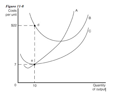
Solved Refer To Figure 11 8 Above To Answer The Following Chegg Com
Figure 11-7 Figure 11-7 shows the cost structure for a firm. 23) Refer to Figure 11-7. When the output level is 100 units average fixed cost is 23) A) $10. B) $8. C) $5. D) This cannot be determined from the diagram.
Solved Figure 11 5 Costs Per Unit Quantity Of Output 4 Chegg Com
2

Refer To Figure 11 5 Identify The Curves In The Diagram Wiring Site Resource
Applied Sciences Free Full Text Effective Safety Assessment Of Aged Concrete Gravity Dam Based On The Reliability Index In A Seismically Induced Site Html

Mechanical Properties Of Circular Nano Silica Concrete Filled Stainless Steel Tube Stub Columns After Being Exposed To Freezing And Thawing
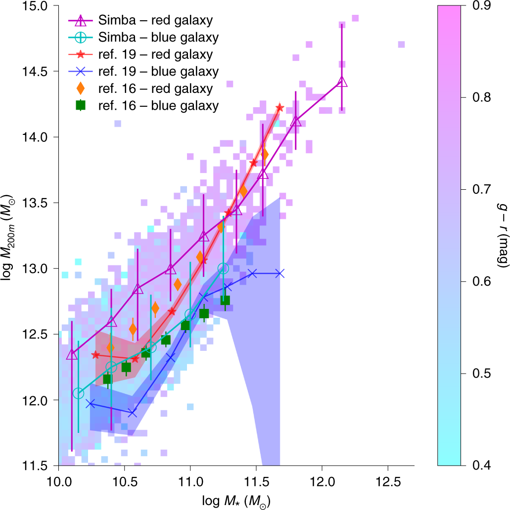
The Origin Of Galaxy Colour Bimodality In The Scatter Of The Stellar To Halo Mass Relation Nature Astronomy

Losing To Blackouts Evidence From Firm Level Data In Imf Working Papers Volume 2018 Issue 159 2018

The Effects Of Heterogeneous Environmental Regulations On Water Pollution Control Quasi Natural Experimental Evidence From China Sciencedirect

Seasonal Variation Of The Indonesian Throughflow In Makassar Strait In Journal Of Physical Oceanography Volume 42 Issue 7 2012
2
Solved Figure 11 5 Costs Quantity Of Output Refer To Figure Chegg Com

Seasonal Variation Of The Indonesian Throughflow In Makassar Strait In Journal Of Physical Oceanography Volume 42 Issue 7 2012

Estimating Photosynthetic Traits From Reflectance Spectra A Synthesis Of Spectral Indices Numerical Inversion And Partial Least Square Regression Fu 2020 Plant Cell Amp Environment Wiley Online Library

Refer To Figure 11 5 Identify The Curves In The Diagram Wiring Site Resource
2
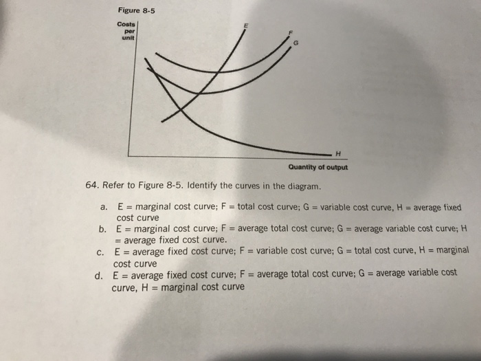
Solved Figure 8 5 Costs E Per Unit G Quantity Of Output 64 Chegg Com
Solved Of Figure 11 1 Total Produet 15 8 Labor Units 36 Chegg Com

Refer To Figure 11 5 Identify The Curves In The Diagram Wiring Site Resource

Refer To Figure 11 5 Identify The Curves In The Diagram Wiring Site Resource
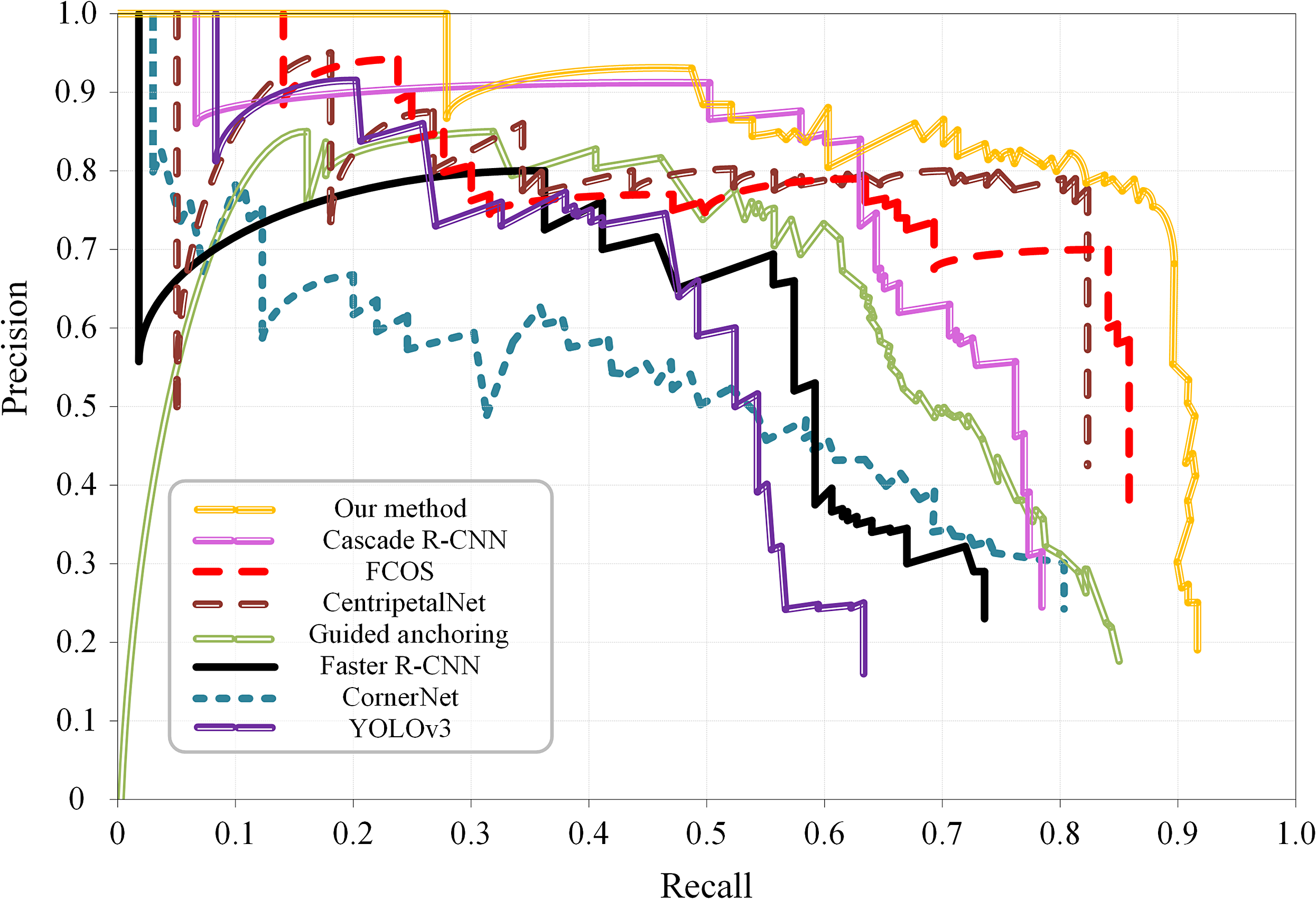
Anchor Free Network With Guided Attention For Ship Detection In Aerial Imagery
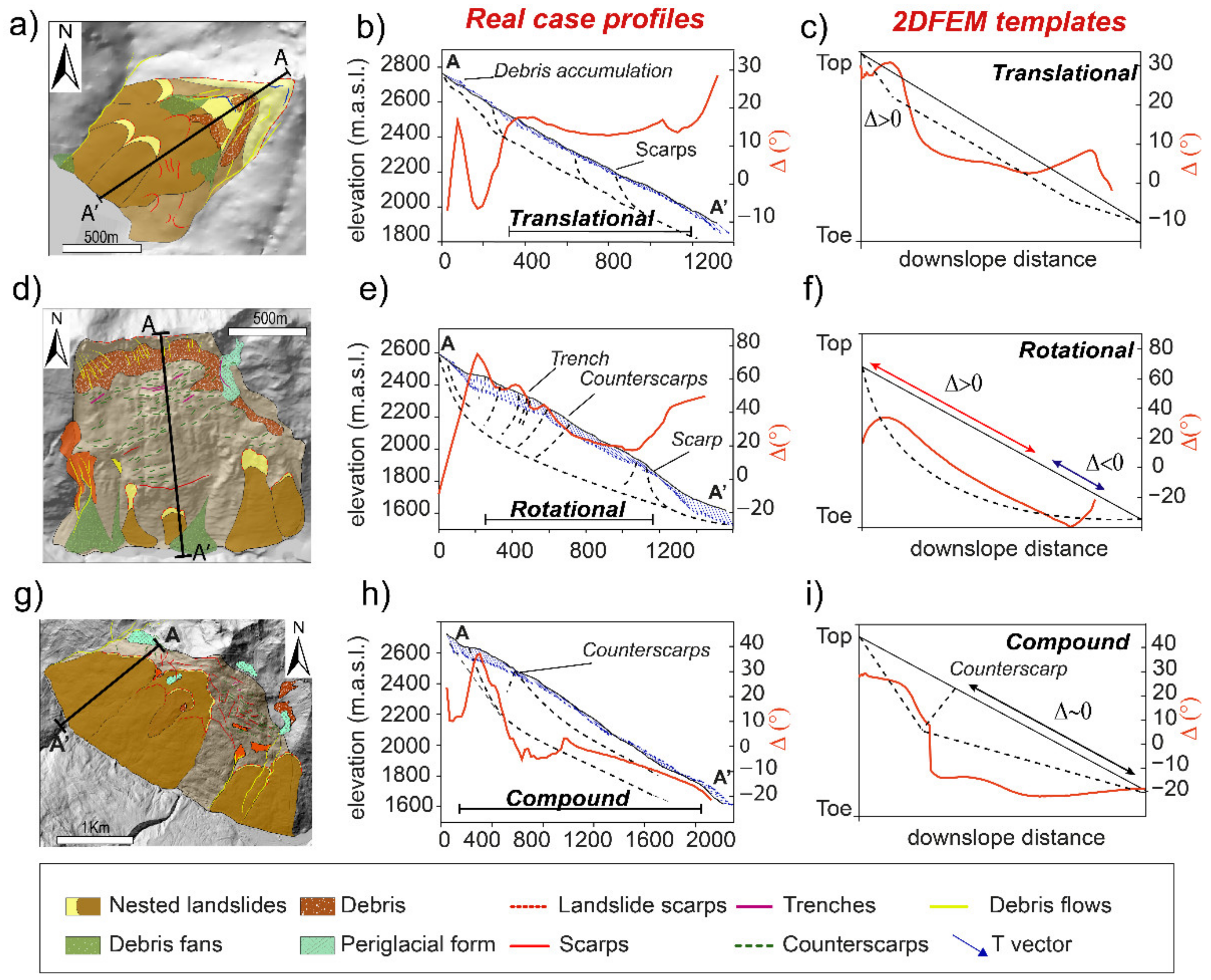
Geosciences Free Full Text Practical Estimation Of Landslide Kinematics Using Psi Data Html

Functional Carbon Quantum Dots For Antitumour Ijn
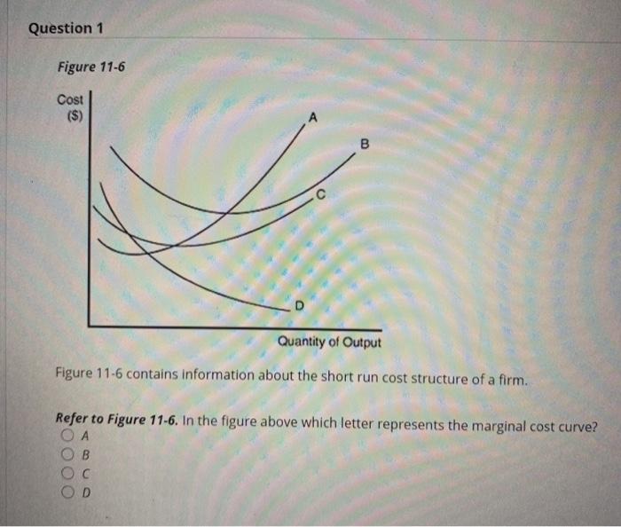
Solved Question 1 Figure 11 6 Cost B Quantity Of Output Chegg Com
Solved Question 1 Figure 11 6 Cost B Quantity Of Output Chegg Com
2

The Annual Cycle Of Sst In The Eastern Tropical Pacific Diagnosed In An Ocean Gcm In Journal Of Climate Volume 11 Issue 5 1998
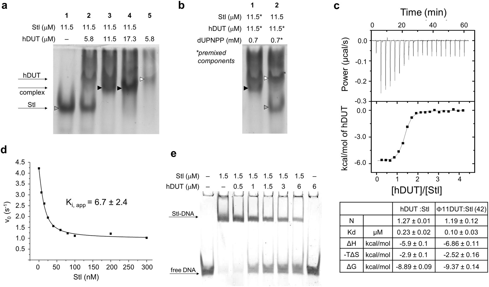
Structural Model Of Human Dutpase In Complex With A Novel Proteinaceous Inhibitor Scientific Reports
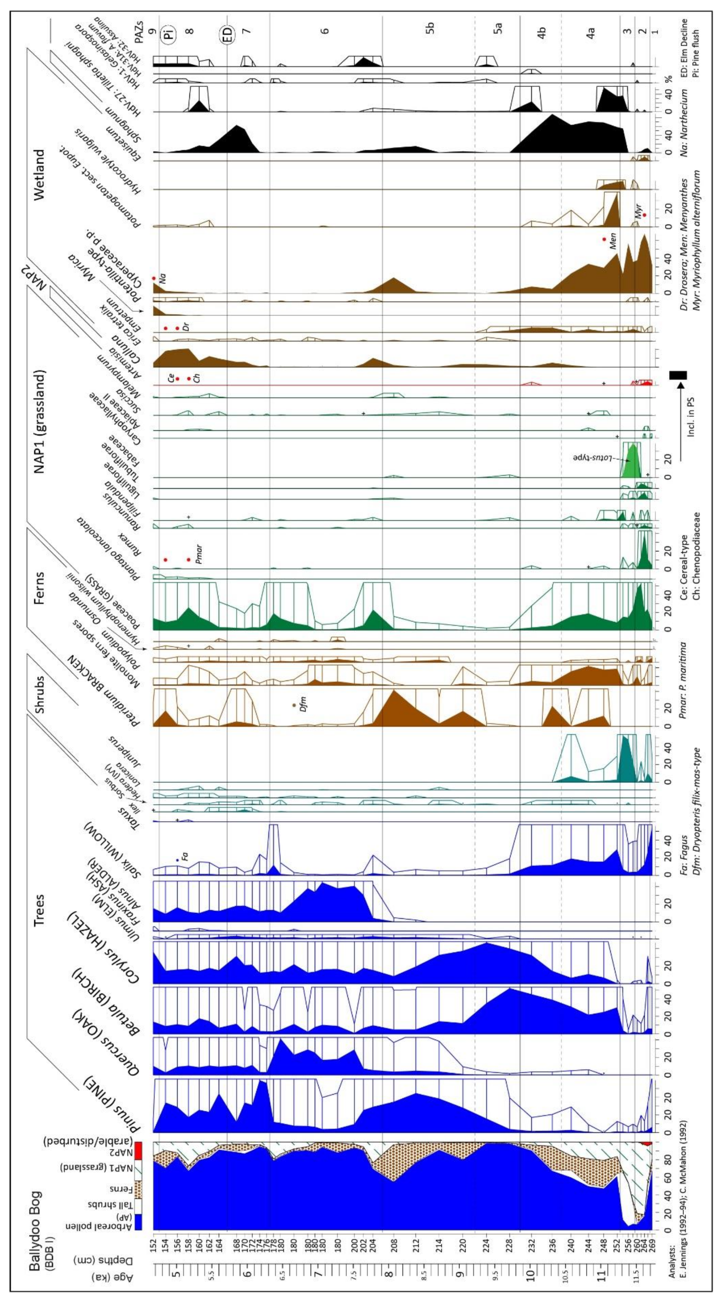
Geographies Free Full Text Holocene Vegetation Dynamics Landscape Change And Human Impact In Western Ireland As Revealed By Multidisciplinary Palaeoecological Investigations Of Peat Deposits And Bog Pine In Lowland Connemara Html
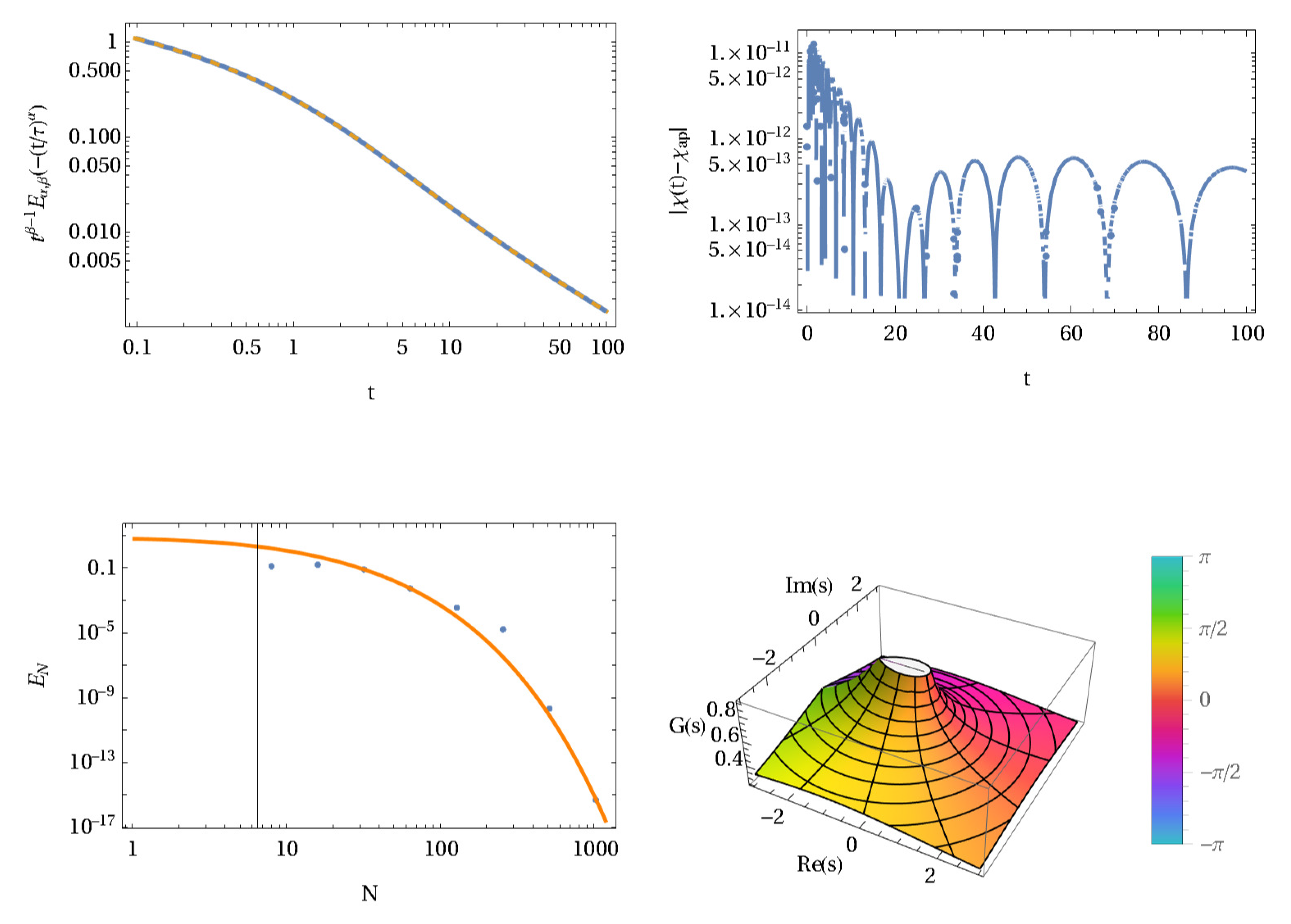
Fractal Fract Free Full Text Sinc Based Inverse Laplace Transforms Mittag Leffler Functions And Their Approximation For Fractional Calculus Html
Solved Figure 11 5 Costs Per Unit G H Quantity Of Output Chegg Com

Refer To Figure 11 5 Identify The Curves In The Diagram Wiring Site Resource

Health Gender And The Household Children S Growth In The Marcella Street Home Boston Ma And The Ashford School London Uk Emerald Insight
Refer To Figure 11 5 Identify The Curves In The Diagram Wiring Site Resource
0 Response to "44 refer to figure 11-5. identify the curves in the diagram."
Post a Comment